Reinforcement Learning-based Hierarchical Seed Scheduling for Greybox Fuzzing

• paper link: https://www.cs.ucr.edu/~heng/pubs/afl-hier.pdf

• video: https://www.youtube.com/watch?v=E90gL7q-IVQ

• code: https://github.com/bitsecurerlab/aflplusplus-hier

Problem to solve

A sensitive (i.e. fine-grained in some sense) coverage metric can select more various seeds as inputs, which helps find out bugs in a program. However, it will cause seed explosion and exceed the fuzzer’a ability to schedule. A fuzzer should consider the balance between exploitation and exploration 1.

Ref to Algorithm 1 in greybox-fuzzing section in this note

Exploitation:

Overhead

• Fuzzing throughput: decides how fast a fuzzer can discover new coverages.

  • examples: AFL uses the fork server and persistent mode to reduce initialization overhead

Exploration:

Coverage (how to add more “diverse” seeds?)

• Test case measurement: e.g. fitness function, that is, what kind of properties the fuzzer can discover (what new coverage introduced by a seed can be viewed as expand the coverage? new edge? new function? new instruction?) (Line 13)

• Seed scheduling criteria: how to prioritize the seeds that are going to be scheduled over other seeds in the pool? (Line 6)

  • example: afl-fast prefers seeds exercising paths that are rarely exercised; libfuzzer prefers seeds generated later during the fuzzing process.

• Seed mutation strategy: how to generate new seeds based on the given old seed? (Line 9)

A few valuable seeds that have led to significantly more new coverage than others in recent rounds encourage to focus on fuzzing them.

Fresh seeds that have rarely been fuzzed may lead to surprisingly new coverage.

The exploration–exploitation dilemma of seed scheduling in a fuzzer can also be modeled as a multi-armed bandit problem, in which

• seeds are regarded as arms (i.e. different slot machines)

• the reward there is the code coverage, which is the objective to maximize

Methodology

Measure the Sensitivity of Different Coverage Metrics

A motivated example: Why a sensetive coverage metric is important in fuzzing

This is a maze shown in line 1-9, steps is a set of instructions to move for each step. When it arrives at #, the player wins.

char maze[7][11] = {
    "+-+---+---+",
    "| |     |#| " ,
    "| | --+ | | " ,
    "| |   | | | " ,
    "| +-- | | | " ,
    "|     |   | " ,
    "+-----+---+" };
int x = 1 , y = 1;
for (int i = 0; i < MAX_STEPS; i++) {
    switch (steps[i]) {
        case 'u': y--; break;
        case 'd': y++; break;
        case 'l': x--; break;
        case 'r': x++; break;
        default :
            printf( "Bad step!" ); return 1;
    }
    if (maze[y][x] == '#') {
        printf( "You win!");
        return 0;
    }
    if (maze[y][x] != ' ') {
        printf( "You lose.");
        return 1;
    }
}
return 1;

If we use symbolic execution/fuzzing to search for a possible path (input),

• Five different inputs: 'a','u','d','l' and 'r' are enough to cover all branches/cases of the switch statement.

• After this, even if the fuzzer can generate new interesting that indeed advance the program’s state towards the goal (e.g., "dd"), the inputs will not be selected as new seeds

• However, if a fuzzer tracks different memory accesses via *(maze+y+x) at line 10 as well, it will be much easier to reach the winning point.

Note

Intuitively speaking, memory access is a more sensitive metric than edge.

Given two coverge metrics \(C_i\) and \(C_j\), we can say that \(C_i\) is more sensitive than \(C_j\) (notated as \(C_i >_s C_j\) ) only if both two conditions holds:

• \(\forall P \in {\cal P}, \forall I_1,I_2 \in {\cal I} , C_i(P,I_1) = C_i(P,I_2) \Rightarrow C_j(P,I_1) = C_j(P,I_2)\): If two inputs lead to the same features (e.g. coverage) under metric \(C_i\), they must have the same features under metric \(C_j\).

• \(\exists P \in {\cal P}, \exists I_1,I_2 \in {\cal I} , C_j(P,I_1) = C_j(P,I_2) \wedge C_i(P,I_1) \ne C_i(P,I_2)\): There must be a pair of inputs that generate no different results under \(C_j\) but can be distinguished under \(C_i\)

For example, edge coverage is more sensitive than basic block coverage. Suppose that two executions go through the same set of basic blocks, but they may reach those blocks from different order/path, so they could cover different edges. However, if two execution cover the identical edges, they must cover the identical basic blocks.

Attention

\(>_s\) is a partial order, two metrics may be not comparable.

Seed Clustering (via Multi-Level Coverage Metrics)

An input \(I\) executed by program \(P\) under \(n\)-dimension metric \(C^n\) produces a sequence of measurements \((M_1,\ldots,M_n)\). For each input/seed, according to the measurments calculated in different levels, it can be classified into a cluster step by step (looks like a decision tree?)

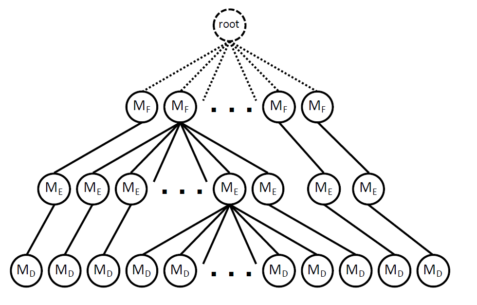
A 3-d metric example: coarse -> fine grained to cluster: function coverage -> edge coverage -> hamming distance. For example, if an input is executed and the measurement is \(M_F\prime\) on function level, it will be first classified by the matched \(M_F\) in the tree and then look onto its \(M_E\) value to see which mid-level node under \(M_F\) can further classified it into a lower level …… At leaf-level, every leaf should be occupied by only one real seed.

From top to down, several metrics with lower to higher sensitivity can be chosen as different levels:

Metric	Notation of metric and measurement	Note
Function	\(C_F\),\(M_F\)	functions that are invoked by an execution
Basic Block	\(C_B\),\(M_B\)	blocks that are exercised by an execution
Edge	\(C_E\),\(M_E\)	edges that are exercised by an execution
Distance	\(C_D\),\(M_D\)	traces conditional jumps (i.e., edges) of a program execution, calculates the hamming distances of the two arguments of the conditions as covered features (difference between the conditional variables when choosing the same edge)
Memory Access *	\(C_A\),\(M_A\)	treats each new index of a memory access as new coverage (not comparable with other metrics in sensitivity)

The input is measured and classified from the least sensitive metric to the most senstive one, forming a hireracy. The process of clustering on input \(I\) can be formalized as:

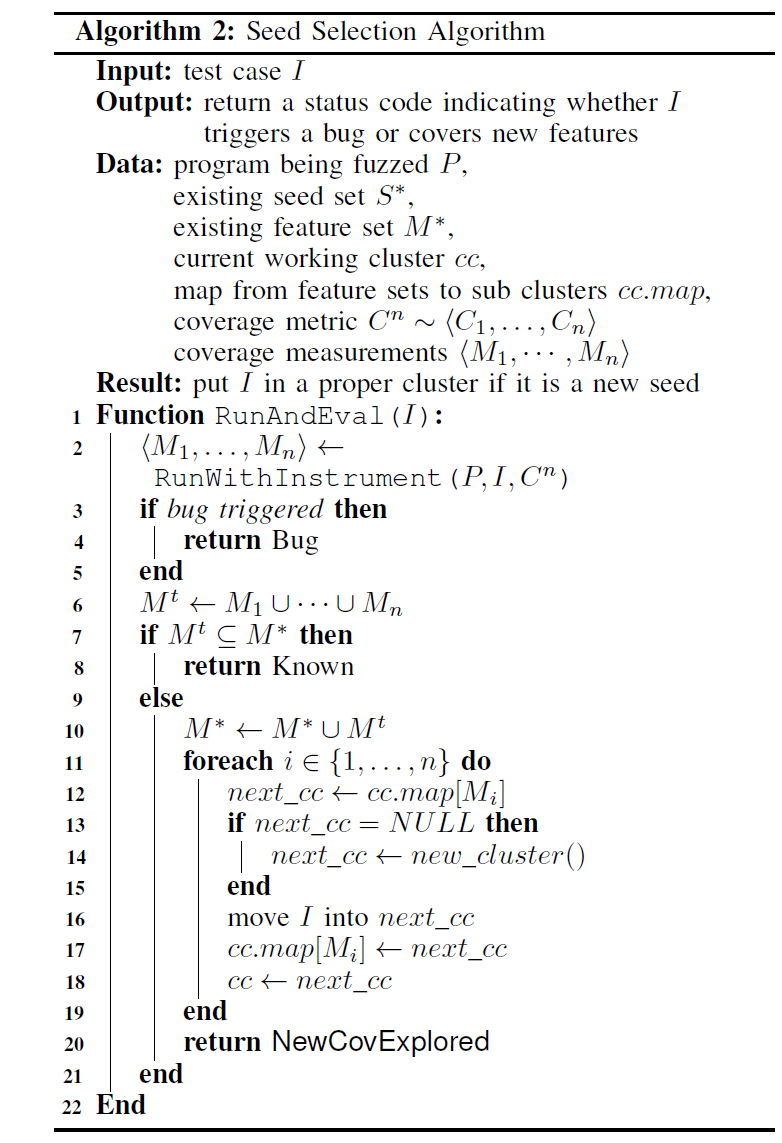
Note: cc_map continually classifies the input to the next-level “cluster” according to its evalution result (measurements). If the input \(I\) can explore a new cluster, it returns NewCovExplored, which doesn’t means more code is covered, sometimes only indicates that new value of coverage appears.

Attention

When two metrics cannot be compared directly in sensitivity, we should cluster a seed with the metric that will select fewer seeds before the one that will select more seeds. - For example, edge coverage and memory access coverage cannot be compared directly, \(C_A\) can generate much more seeds than \(C_E\) via observation, so \(C_A\) should come after \(C_E\) in the tree structure.

Scheduling against A Tree of Seeds

Note

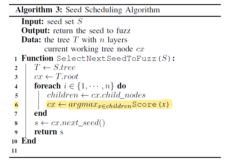
A traditional MAB problem assumes a fixed number of arms (nodes in our case) so that all arms can get an estimation of their rewards at the beginning. But for seed scheduling, the number of nodes grows as more and more seeds are generated. So the new added seed will be assigned a rareness value as its intial score.

To select a seed from the tree: start from the root node, select the child node with the highest socre (score is calculated based on the coverage measurements), until the last layer (real seeds).

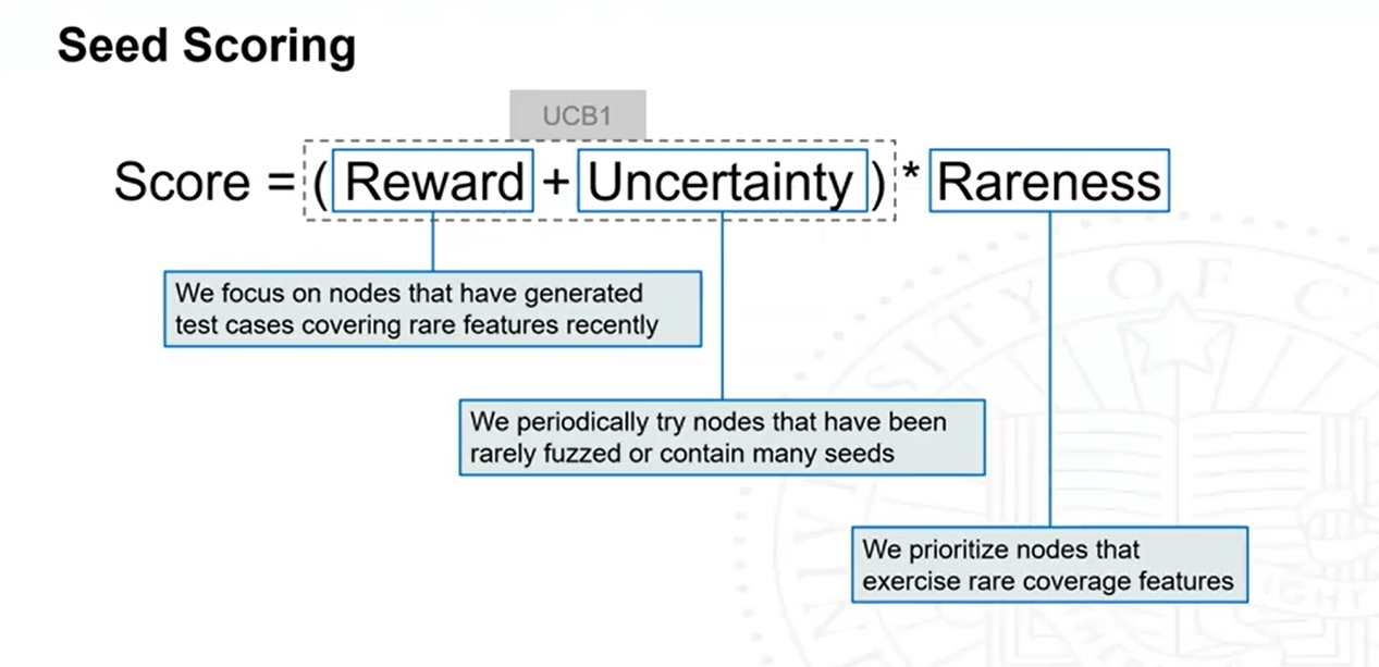
The fuzzing performance (score) of a node \(a\) is estimated by UCB12 formula:

\[FuzzPerf(a) = Q(a) + U(a)\]

• \(Q(a)\): empirical average of fuzzing rewards that \(a\) obtains so far

• \(U(a)\): radius of the upper confidence interval

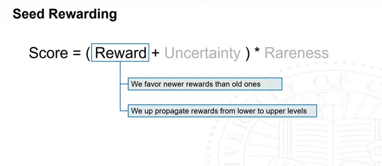
The overall score is:

\[Score(a) = Rareness(a) \times FuzzPerf(a)\]

Formula reduction & Detailed definition

Notation	Explanation
num_hits(F)	the number of test cases ever generated that cover the feature F
rareness(F)	1/num_hits(F)
fcov[s,l,t]	a feature set that consists of all features covered at levels l by
SeedReward(s,l,t)	The max rareness value of F in fcov[s,l,t]
\(Reward(a^l,t)\)	assume \((a^1,\ldots, a^{n+1})\) is the sequence of nodes selected at round \(t\), the reward of the scheduling node \(a^l\) at round \(t\) is caclculated by the geometric mean of SeedReward the following (lower) nodes (i.e. \(\sqrt[n-l+1]{\prod_{k=l}^{n} SeedRewards(s,k,t)}\))
Q(a,t)	\(\frac{Reward(a,t)+w\times Q(a,t^\prime) \times \sum_{p=0}^{N[a,t]-1}{w^p}}{1+w\times\sum_{p=0}^{N[a,t]-1}{w^p}}\) it progressively decreases the weight to the previous mean reward in order to give higher weights to newer rewards, discount factor \(w\) is empirically set to 0.5.
U(a)	\(C \times \sqrt{\frac{Y[a]}{Y[a^\prime]}} \times \sqrt{\frac{log N[a^\prime]}{N[a]}}\), \(Y\) denotes number of seeds in the cluster, \(N\) denotes the times has been selected so far
SeedRareness(s,l)	\(\sqrt{\frac{\sum_{F \in C_l(P,s)}^{}{rareness^2[F]}}{|\{F:F \in C_l(P,s)\}|}}\)
\(Rareness(a^l)\)	SeedRareness(s,l)

At the end of each round of fuzzing, nodes along the scheduled path will be rewarded based on how much progress the current seed has made in this round. (whether there are new coverage features exercised by all the generated test cases)

• seeds that perform well are expected to have increased scores for competing in the following rounds

• seeds making little progress will be de-prioritized.

Evaulation & Results

• Benchmark: DARPA Cyber Grand Challenge (CGC) + Google FuzzBench

• Implementations: built on AFL/AFL++ QEMU-MODE

• Performance

  • crashes more binaries and faster

  • generally achieved more code coverage and achieved the same coverage faster

---

1

This slides explains more basic knowledge on exploitation/exploration trade-off and multi-armed bandit problem.

2

This page provides a visualization and explanation of UCB1 algorithm in multi-armed bandit problem.

A Survey on Fuzzing   A Survey on Security of Automatic Generated Code